Update rules for least squares

Introduction

In this project, I will explore fitting a running linear model as well as running predictions.

During my bachelor’s project, I focused on the prediction of time series. The model I used was fitted using least squares. I worked with FFP3, which is implemented in R.

At that time, I used the Forecast package but ended up implementing the estimator from the ground up. As I have improved my programming and mathematical skills, I thought it would be fun to revisit this problem and see if I could develop a better solution.

Rob who wrote FFP3, has a blog their i sais their is trick to speeding op the calculation of rolling predition for AR process, and I think I figured it out.

Lest squres can be written as

\[\underset{\beta}{argmin} ||Y-X\beta||^2\]

Since this is a linear function the problem above i convex with one uniq closed form solution

\[\hat{\beta}=(X^TX)^{-1}X^TY\]

Running Prediction

When using a running model, a simple solution is to add a new data point and fit the model again. This approach works but is not very efficient.

Instead, let’s consider whether we can update the \(\beta\) estimates directly.

One option is the Recursive least squares filter

A simpler version is using Sherman–Morrison formula

Let’s explore how (Sherman–Morrison) can be used.

Let \(x[i]\) represent the i-th index of the vector.

For \(XX^T\) a rank-1 update can be expressed as:

\[(X_{new}X_{new}^T)=(X_{old}^TX_{old})+x_{new}^Tx_{new}\]

This becomes clear when the product is written out explicitly.

Look at \((X^TX)[j,g]=x_j^Tx_g\) So \(\sum_{i=1}^{n}x_{j}[i]x_{g}[i]\)

Next, consider a given entry in the inner product. \((X_{old}X_{old}^T)_{[j,g]}=x_j^Tx_g\) So \(\sum_{i=1}^{n}x_{j}[i]x_{g}[i]\)

Now look at.

\((X_{new}X_{new}^T)[j,g]=(\sum_{i=1}^{n}x_{j}[i]x_{g}[i])+x_{new}[j]x_{new}[g]\)

use Sherman–Morrison formula

For the update of \((X^TX)\)

\[(X_{new}^TX_{new})^{-1}=(X_{old}^TX_{old}+x_{new}^Tx_{new})^{-1}=(X_{old}^TX_{old})^{-1}-\frac{(X_{old}^TX_{old})^{-1}x_{new}^Tx_{new}(X_{old}^TX_{old})^{-1}}{1+x_{new}(X_{old}^TX_{old})^{-1}x_{new}^T}\]

Let’s look at the nex part of the expresion

For \(B=X^TY\) the udpate rule is \[B=(X_{new}^TY_{new})=(X_{old}^TY_{old})+x_{new}*y_{new}\]

note here that \(y_{new}\) act as a scale

Use Cases

Rolling prediction can be used for the evaluation of time series.

However, these techniques can also be used for the quick implementation of a sliding window estimator or to update a linear model as new data arrives. Additionally, this method provides a fast approach for leave-one-out evaluation of predictive strength.

I will create one implementations, where I use this for rolling prediction.

The method could be used for making a implements of a sliding window.

For the sliding window, it is necessary not only to add the new row but also to remove the old one.

import numpy as np
import unittest

def get_rank_updated_matrix(A: list, v: list, u: list):
    return A + v.T @ u
def test_get_rank_updated_matrix():
    A_test=np.array([[1,0],[0,1]])
    v_test=np.array([[1,1]])
    u_test=np.array([[1,1]])
    assert (np.all(get_rank_updated_matrix(A_test,v_test,u_test)==np.array([[2, 1], [1, 2]])))
    return
test_get_rank_updated_matrix()


def test_get_inverse_updated_matrix_remove_row():
    X_T_inner_X_inverse_test=np.array([[1,1],[1,1]])
    x_test=np.array([[1,1]])
    assert np.all(get_inverse_updated_matrix(X_T_inner_X_inverse_test,x_test)==np.array([[1,1],[1,1]])+4/5)
    return

def get_inverse_updated_matrix_remove_row(X_T_inner_X_inverse: list, x: list):
    return X_T_inner_X_inverse + X_T_inner_X_inverse @ (x.T @ x) @ X_T_inner_X_inverse / (1 + x @ X_T_inner_X_inverse @ x.T)


def get_inverse_updated_matrix(X_T_inner_X_inverse: list, x: list):
    return X_T_inner_X_inverse - X_T_inner_X_inverse @ (x.T @ x) @ X_T_inner_X_inverse / (1 + x @ X_T_inner_X_inverse @ x.T)

def test_get_inverse_updated_matrix():
    X_T_inner_X_inverse_test=np.array([[1,1],[1,1]])+4/5#np.array([[1,1],[1,1]])
    x_test=np.array([[1,1]])
    assert np.all(get_inverse_updated_matrix_remove_row(X_T_inner_X_inverse_test,x_test)==np.array([[1,1],[1,1]]))
    return


def get_least_sqrd_closed_form_parameter(X: list, Y: list):
    return np.linalg.inv(X.T @ X) @ X.T @ Y

def test_get_least_sqrd_closed_form_parameter():
    X_test=np.array([[1,0],[0,1]])
    Y_test=np.array([[1],[1]])
    assert np.all((get_least_sqrd_closed_form_parameter(X_test,Y_test))==[[1],[1]])
    return
test_get_least_sqrd_closed_form_parameter()

def get_least_sqrd_A_B_parameter(A: list, B: list):
    return A @ B

def test_get_least_sqrd_A_B_parameter():
    A_test=np.array([[1,0],[0,1]])
    B_test=np.array([[1,0],[0,1]])
    assert np.all(get_least_sqrd_A_B_parameter(A_test,B_test)==[[1,0],[0,1]])
    return
test_get_least_sqrd_A_B_parameter()

def get_matrix_update_B(B: list, x: list, y:float):
    return B + x.T *y

def test_get_matrix_update_B():
    B_test=np.array([[1,1]])
    x_test=np.array([[1,1]])
    y_test=2.0
    assert np.all(get_matrix_update_B(B_test,x_test,y_test)==np.array([[3.0,3.0]]))
    return
test_get_matrix_update_B()

def get_matrix_update_B_remove_row(B: list, x: list, y:float):
    return B - x.T *y

def get_matrix_update_B_remove_row():
    B_test=np.array([[1,1]])
    x_test=np.array([[1,1]])
    y_test=1.0
    assert np.all(get_matrix_update_B_remove_row(B_test,x_test,y_test)==np.array([[0.0,0.0]]))
    return
test_get_matrix_update_B()

def get_prediction(A, B, X):
    return X@get_least_sqrd_A_B_parameter(A, B)

def test_get_prediction():
    x_test = np.array([[1, 0], [1, 1]])
    y_test = np.array([[1], [2]])
    A_test = np.linalg.inv(x_test.T @ x_test)
    B_test = x_test.T @ y_test
    assert np.all((get_prediction(A_test, B_test, np.array([[1, 2]])))==[[3]])
test_get_prediction()

def rolling_prediction(x: list, y: list, starting_length: int):
    # Ensure x is 2D array with shape (n_samples, n_features)
    x_array = np.array(x).reshape(-1, 1) if len(np.array(x).shape) == 1 else np.array(x)
    y_array = np.array(y).reshape(-1, 1) if len(np.array(y).shape) == 1 else np.array(x)
    
    length = len(x_array)
    prediction = np.zeros(length - starting_length)
    los_score = np.zeros(length - starting_length)

    # Initialize A and B matrices
    initial_x = x_array[:starting_length]
    initial_y = y_array[:starting_length]
    
    A = np.linalg.inv(initial_x.T @ initial_x)
    B = initial_x.T @ initial_y

    # Initial prediction
    next_x = x_array[starting_length].reshape(1, -1)  
    prediction[0] = get_prediction(A, B, next_x)
    los_score[0] = y_array[starting_length] - prediction[0]
    
    # Rolling update for predictions and loss scores
    
    ind = starting_length + 1
    current_x = x_array[ind].reshape(1, -1)  
    for i in range(length - starting_length - 1): 
        ind = starting_length + i
        current_x = x_array[ind].reshape(1, -1) 
        # Update matrices
        A = get_inverse_updated_matrix(A, current_x)
        B = get_matrix_update_B(B, current_x, float(y_array[ind]))
        # Make prediction for next point
        next_x = x_array[ind + 1].reshape(1, -1)  
        prediction[i + 1] = get_prediction(A, B, next_x)
        los_score[i + 1] = y_array[ind + 1] - prediction[i + 1]
    return {"prediction": prediction, "los_score": los_score}

Testing the Application

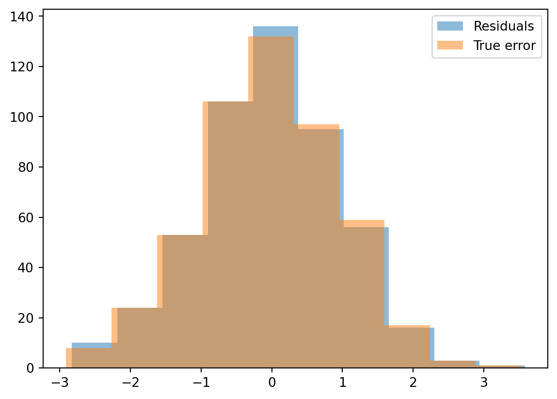
Since the underlying model is not changing, this provides a straightforward way to test the model. The residuals should closely resemble the errors.

However, they will not be identical, as this would require the coefficients to be perfectly accurate.

import warnings
warnings.filterwarnings("ignore")
#Dianostic plot 
import matplotlib.pyplot as plt

start_val=500
x = np.random.rand(1000)  
error=np.random.normal(size=1000)  
y = 2*x + error

# Run the prediction
result = rolling_prediction(x, y, start_val)


plt.hist(result['los_score'],alpha=0.5)

plt.hist(error[(start_val):],alpha=0.5)
plt.legend(["Residuals", "True error"])
plt.show()

When the Application Fails

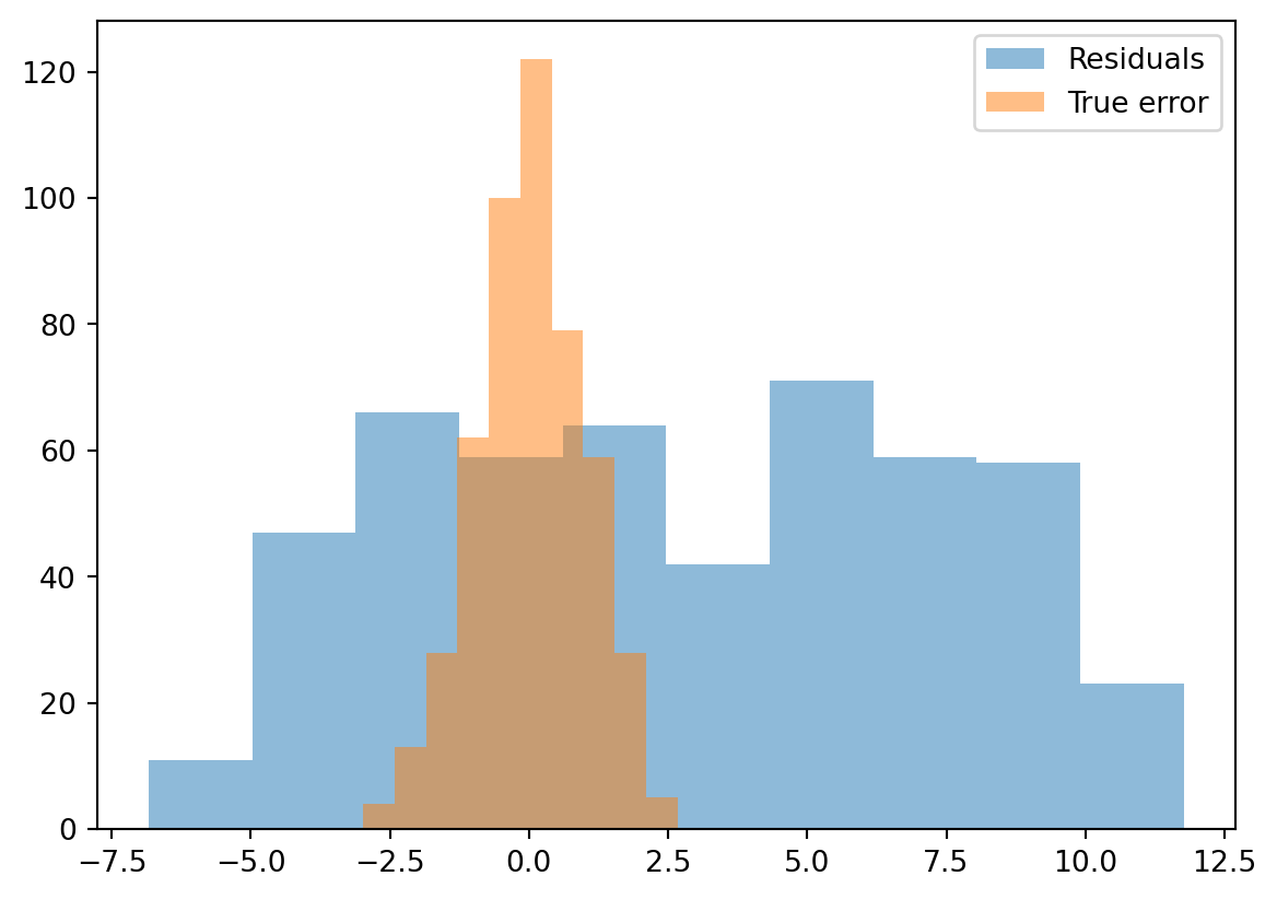
The reader should note that I have not included an intercept in the data-generating process. Below, I have conducted the same test, but this time I have added a constant to the expression.

import warnings
warnings.filterwarnings("ignore")
#Dianostic plot 
import matplotlib.pyplot as plt

start_val=500
x = np.random.rand(1000)  
error=np.random.normal(size=1000)  
y =10+ 2*x + error

# Run the prediction
result = rolling_prediction(x, y, start_val)


plt.hist(result['los_score'],alpha=0.5)

plt.hist(error[(start_val):],alpha=0.5)
plt.legend(["Residuals", "True error"])
plt.show()

As can be see now the aplication fails.

This can be fixed by adding a column of ones to the model matrix. I would also need to update all the functions to accommodate this change. Without adjusting for this, the dimensions will not match when adding the point to the inverse.

I will stop the project here. This was intended to be a small NumPy project. If I were to create functions that allow specifying a model, I might develop it more properly and let the user specify the model through an expression, similar to how linear models are specified in R. Since all model specifications in linear models are based on modifying the model matrix, this could provide flexibility.