Sequential Hypothesis Testing and Safe Anytime Inference

Preface to This Project

This project was one of those rabbit-hole endeavors. I wanted to learn about A/B testing, which turned out to be a straightforward hypothesis test with some power calculations.

Interestingly, the calculations for power analysis were concepts I had already learned during my bachelor’s degree. So, I decided to explore some newer methods instead. That led me to sequential testing—a fascinating field. It’s this intriguing mix of betting strategies, martingales, and a lot of other fun concepts.

I’m mostly writing this project for myself, so I have something to work on and a way to document my learning process. But if someone happens to stumble across this, they should be aware that it can get a bit technical. I’ve included references to the math so I can easily find it again, and I’ve conducted a few small simulation studies. These simulations help me get a sense of the performance of the methods while also allowing me to bend the assumptions a little to see what happens.

Introduction

So in this project i am looking in to Wald’s Sequential Probability Ratio Test also called SPRT and some variants like mSPRT. The reason i want to learn this, is sequsial testing method. This is used to make live monotering of of Hyposis. It eliminates the need for power calucluastions, insted the parameters \(\alpha\) and \(\beta\) is chosen/specified befor the start of the experiment and the sampling proces gones on, until the hyposis can be confirmed or rejected. This is more inline with how i would want to conduct experimetns, their is some simularty to stocastic bandit, where agent tryes to optimize reward will they learn, for SPRT, the goal is to stop the experiment when a hypsis can be confirmed ore rejected.

The use cases for this live experiment such as A/B testing, but some mention trials aswell, I would think it would be hard to get aproved.

These test is based on significance and p-values, with the subject matter focusing on hypothesis testing. I assume the reader is already familiar with this concept, as I typically write these short notes for my personal reference. The concept of significance can be explained by the user selecting an \(\alpha\) level, which defines the desired confidence level or coverage. This can be thought of as representing the user’s tolerance for making an error. In many research fields, a common choice is \(\alpha = 0.05\), which corresponds to tolerating a 5% error rate. For this experimental design, the goal is that if 100 experiments are conducted, we would expect the correct hypothesis to be confirmed approximately \((1 - \alpha) \times 100\) times.

So why use these Sequential test rather than normal likelihod ratio test og confiens intervalls and the reason is peeking, wish we will get into later.

Power calulation

This project started with me looking into power calculations. In this section i go throug how to make the power caluculations and look into what happens if on peeks.

So the power calulation works by the user setting the minimum effect they would want the calculate, and tolarance for type 1 error \(\alpha\) and tolerance for type 2 \(\beta\).

Let \(X=x_1,\dots,x_n\) be the data depend if \(x_i\sim \mathbb{N}(\mu,\sigma^2)\) ore if mean \(\bar{X}\sim \mathbb{N}(\mu,\sigma^2)\), the last come often from the law of large number. One can use this method. I am not goin in to much in detail here, relly like this explation. The pivot is showen in the calulaten’s.

Formally

Let \(H_0\) be the null and let \(H_1\) be other hyposis

\(\alpha\) is the proberbillaty of making a type one error meaning

\(P(acepting\: H_1\: when\: H_0\: is\: true)\)

\(\beta\) is the probillaty of type 2 error

\(P(acepting\: H_0\: when\: H_1\: is\: true)\)

If the distribtion is nice meaning law of large number insure it conveges to normal distribuion.

\[n\geq 2(\frac{\phi^{-1}(1-\alpha-\phi^{-1}(1-\beta)}{\Delta/\sigma})^2\]

\(\phi^{-1}\) is the inverse cumulative standard normal distribution,

\(\Delta\) is the abeslut differnece in effect betwwen the null \(H_0\) and \(H_1\).

\(\sigma\) is the variance.

Peeking

Peeking is when a one looks at the data as they come in, using standart hyposis test method, and make a conclusion if they dont see a effect. The problem is that it destrou the coverage gaurenty. So if one look at the data as they flow in and end the experiment and before if their is no significans.

This idear of if we have hundret experiement, in \((1-\alpha)*100\) the right hypothesis identified is not valid.

Below i have made some small simulations to ilustrate the problem

\(A=a_1,\dots,a_n\) and \(B=b_1,\dots,b_n\) let \(a_i\) and \(b_i\) iid and let \(a_i\sim\mathbb{N}(0,1)\) and \(b_i\sim\mathbb{N}(0,1)\).

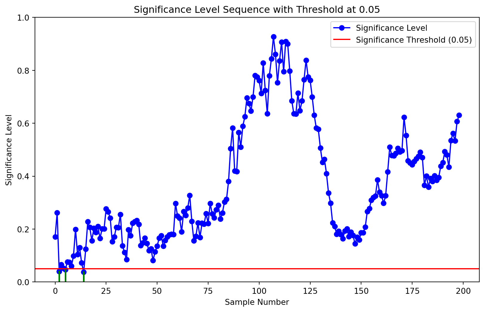
Since \(A\) and \(B\) has the same distribuion their is no effect. This is sometime calle a A/A test. Sometimes this is used to test method in a live environment. If a useres test method, they should get the type 1 error cover from this.

At each point the simulation will draw with no replacment from A ore B calulat the p values and see if the true mean is in the confiden intervall.

import random
import numpy as np
import matplotlib.pyplot as plt
from scipy.stats import norm
random.seed(42)
# Parameters
n = 100  # Number of samples in A and B
num_simulations = 1  # Number of simulations
alpha = 0.05  # Significance level
true_mean = 0  # True mean to check against
variance=1 # varince know
a=np.random.normal(true_mean,variance,n) # draw
b=np.random.normal(true_mean,variance,n) # draw

def get_sigficanlevet(A:list,B:list,A_variance:float=1,B_variance:float=1):
    mean_A=np.mean(A)
    mean_B=np.mean(B)
    Z = (mean_A - mean_B) / np.sqrt(A_variance / len(A) + B_variance/ len(B))
    p_value = 2 * (1 - norm.cdf(abs(Z)))
    return p_value


def get_significant_seq(A: list, B: list, A_variance: float = 1, B_variance: float = 1):
    # Initialize an empty list to store the significant values
    sig_seq = []

    # Create copies of A and B for sampling without replacement
    A_copy = np.copy(A)
    B_copy = np.copy(B)

    # Initialize vectors for the selected samples
    A_vector = []
    B_vector = []

    # Sample the first element from A and B
    A_vector.append(A_copy[0])
    A_copy = np.delete(A_copy, 0)

    B_vector.append(B_copy[0])
    B_copy = np.delete(B_copy, 0)

    # Initial significance level calculation
    sig_seq.append(get_sigficanlevet(A_vector, B_vector))  # Assuming this function exists

    # Run the loop until both lists are empty
    while len(A_copy) > 0 or len(B_copy) > 0:
        # Randomly choose whether to sample from A or B
        if np.random.rand() > 0.5 and len(A_copy) > 0:
            A_vector.append(A_copy[0])  # Append the first element from A
            A_copy = np.delete(A_copy, 0)  # Remove the sampled element from A
        elif len(B_copy) > 0:
            B_vector.append(B_copy[0])  # Append the first element from B
            B_copy = np.delete(B_copy, 0)  # Remove the sampled element from B
        
        # Calculate and store the significance level at this step
        sig_seq.append(get_sigficanlevet(A_vector, B_vector))  # Assuming this function exists

    return sig_seq


def plot_significance_seq(sig_seq):
    # Plot the significance sequence
    plt.figure(figsize=(10, 6))
    plt.plot(sig_seq, marker='o', linestyle='-', color='b', label='Significance Level')
    
    # Add horizontal line at y=0.05 for the threshold
    plt.axhline(y=0.05, color='r', linestyle='-', label='Significance Threshold (0.05)')
    
    # Add small green line segments for significance values below 0.05
    for i, value in enumerate(sig_seq):
        if value < 0.05:
            plt.plot([i, i], [0, value], color='green', lw=2)  # Line from 0 to the value

    # Set limits for the y-axis between 0 and 1
    plt.ylim(0, 1)
    
    # Adding labels and title
    plt.xlabel('Sample Number')
    plt.ylabel('Significance Level')
    plt.title('Significance Level Sequence with Threshold at 0.05')
    
    # Adding a legend
    plt.legend()

result=get_significant_seq(a,b)
plot_significance_seq(result)

As can be see from the plot the p values goes up and down doing the experiment, So if one was to stop the experiement when the p value cross a threshold. The cover is not correct, this means in this case that tyoe 1 error alot higer than one exptes.

So let’s look at how the coverage is affected by the peaking. Belove i have made small simulation that corespond to making the plot above a 1000 times and with a p value \(0.05\).

I simulate two draws from the same distribution and check if there is a significant difference between them. If a significant difference is found, I stop the experiment and count it as a success. If no significant difference is found, the experiment continues with a new draw, and the same test is conducted. I repeat this process for 100 draws and 1000 experiments. Finally, I sum the number of experiments that show a significant result and divide this sum by the total number of experiments (1000) to calculate the proportion of significant results.

import numpy as np
import matplotlib.pyplot as plt
from scipy.stats import norm



def get_sigficanlevet(A:list,B:list,A_variance:float=1,B_variance:float=1):
    mean_A=np.mean(A)
    mean_B=np.mean(B)
    Z = (mean_A - mean_B) / np.sqrt(A_variance / len(A) + B_variance/ len(B))
    p_value = 2 * (1 - norm.cdf(abs(Z)))
    return p_value


def run_significant_seq(A: list, B: list, A_variance: float = 1, B_variance: float = 1):
    # Initialize an empty list to store the significant values

    # Create copies of A and B for sampling without replacement
    A_copy = np.copy(A)
    B_copy = np.copy(B)

    # Initialize vectors for the selected samples
    A_vector = []
    B_vector = []

    # Sample the first element from A and B
    A_vector.append(A_copy[0])
    A_copy = np.delete(A_copy, 0)

    B_vector.append(B_copy[0])
    B_copy = np.delete(B_copy, 0)
    
    sig_erro=0
    # Run the loop until both lists are empty
    while len(A_copy) > 0 or len(B_copy) > 0:
        # Randomly choose whether to sample from A or B
        if np.random.rand() > 0.5 and len(A_copy) > 0:
            A_vector.append(A_copy[0])  # Append the first element from A
            A_copy = np.delete(A_copy, 0)  # Remove the sampled element from A
        elif len(B_copy) > 0:
            B_vector.append(B_copy[0])  # Append the first element from B
            B_copy = np.delete(B_copy, 0)  # Remove the sampled element from B
        
        # Calculate and store the significance level at this step
        if(get_sigficanlevet(A_vector, B_vector)<0.05):
            sig_erro=1
            break 
    return sig_erro



n = 100  # Number of samples in A and B
num_simulations = 1000  # Number of simulations
alpha = 0.05  # Significance level
true_mean = 0  # True mean to check against
variance=1 # varince know

estimated=[]
for i in range(1,num_simulations):
    a=np.random.normal(true_mean,variance,n) # draw
    b=np.random.normal(true_mean,variance,n) # draw
    estimated.append(run_significant_seq(a,b))

print("cover")
print(np.mean(estimated))

cover
0.38738738738738737

For these settings, I usually obtain an estimate of around 0.4, which, to me, seems high. Remember, this should be the Type 1 coverage rate, so around 0.05. In practice, a person would likely not peek at the data every time a new point arrives. This is merely intended to illustrate the problem of peeking.

If peeking causes problems, the solution seems obvious: avoid peeking. However, in practice, people often do.

The literature on the method introduced below discusses designing systems to account for user behavior. This includes cases where users receive credit for findings, even when peeking leads to results that may not be valid.

The goal is to develop mathematical models that mitigate the problem of peeking. Another approach is preregistration. That said, there are many valid reasons to evaluate results as data comes in and to stop when a clear conclusion can be drawn.

Betting for Hypothesis Testing.

The main idea behind betting in hypothesis testing is to reframe the problem of hypothesis testing into a game.
In this game, if the null hypothesis is true, there should be no strategy to consistently earn money. However, if one starts making money by betting against the null hypothesis, at some point it becomes highly unlikely that the null is true, allowing one to reject it.

Let us think about this.
To give an example, imagine you are betting on the outcomes of two coin flips. You can bet on whether the coins match (both heads or both tails) or not. The coins may either be fair or have a matching bias, meaning both coins have a higher probability of landing on heads or tails.

If you guess correctly, you double your money; if you guess incorrectly, you lose your money. Note that there are only two hypotheses here. A rational player would not bet all their money but rather a fraction of it. A small note: The optimal fraction can be determined by optimizing log wealth. I won’t go into the details here, but this approach is widely used in the e-variable literature, which I refer to at the end.

Let \(H_0\) represent the null hypothesis that there is no difference between the coins, meaning they are fair. For a fair game, \(P(x = \text{match}) = 0.5\), and there is no strategy to earn money. You could always bet “match,” always bet “no match,” or condition your bets on the previous outcome—it doesn’t matter. This also means there are no consequences to betting on \(H_1\).

Now, if the coins are biased, say \(P(x = \text{match}) = 0.6\), the optimal strategy is to always bet on “match”.

The above fair game is a sup martingale meaning meaning that the expected winnings at any point in time are equal to or less than what one has currently, and the value of the wealth process is always positive.

Let \(M_t\) represent the wealth process in the game, i.e., the amount of money one has at time \(t\).

Ville’s inequality states that

\[\mathbb{P}\left( \exists t \geq 1 : M_t \geq x \right) \leq \frac{\mathbb{E}[M_0]}{x}\]

This means that there is a set probability that \(M_t\) will cross \(x\) over the entire duration of the process, assuming the game is fair.

Now, if the game is not fair, at some point we will win enough money to cross the threshold defined by Ville’s inequality. On the other hand, if the game is fair, with some probability (determined by \(\alpha\)), \(M_t\) will still cross the inequality.

This provides the correct control for the null hypothesis, but it holds over the entire process.

sequential probability ratio test (SPRT)

A little more formal explanation of the SPRT:
Here, we are only looking at two hypotheses and their corresponding points:

• \(H_0: \theta = \theta_0\), where \(p(x_i)\) is the distribution under the null hypothesis.
  
• \(H_1: \theta = \theta_1\), where \(q(x_i)\) is the distribution under the alternative hypothesis.

We begin with a wealth of one.

Under the null hypothesis, the expectation of the likelihood ratio is given by:

\[ \mathbb{E}_{q(x)}( \frac{q(X_i)}{p(X_i)}) = \int \frac{p(x)}{q(x)} q(x) \, dx = \int p(x) \, dx = 1 \]

The wealth can be written as:

\[ M_t = \prod_{i=1}^{T} \frac{q(X_i)}{p(X_i)} \]

This is a submartingale, and by using Ville’s inequality, we obtain a probability guarantee for the entire process.

Under the alternative hypothesis, the inverse of the likelihood ratio will be a submartingale, leading to two thresholds: one for rejecting the null hypothesis \(H_0\) and one for rejecting \(H_1\).

\(a\approx \frac{\beta}{1-\alpha}\) and \(b \approx \frac{1-\beta}{\alpha}\)

if \(M_t \geq b\) accept \(H_1\) if \(M_t \leq a\) accept \(H_0\)

Otherwise sample a new point.

Notice how simple the theory is here.

Wiki is good reference for this.

Simulation

Below i have made small simulation of the the fair game desciped above and the SPRT. both coins af fair meaning their is \(P(X=head)=0.5\) for both \(\alpha = 0.05\)

import numpy as np

# Variables for the experiment
p_coin_1 = 0.5
p_coin_2 = 0.5

# Probability of match and no match
p_match = (1 - p_coin_1) * (1 - p_coin_2) + p_coin_1 * p_coin_2
p_no_match = 1 - p_match

# Hypotheses
match = 0.5  # Null hypothesis
alternative_hypothesis = 0.7  # Alternative hypothesis

# Tolerances
alpha = 0.05  # Type I error
beta = 0.20  # Type II error

# Thresholds
a = np.log(beta / (1 - alpha))
b = np.log((1 - beta) / alpha)

# Make button


def ber_llr(h_0, h_1, outcome):
    """
    Calculate the log-likelihood ratio for a Bernoulli outcome.
    
    Args:
        h_0: Null hypothesis probability
        h_1: Alternative hypothesis probability
        outcome: Observed outcome (0 or 1)
        
    Returns:
        Log-likelihood ratio for the given outcome.
    """
    return np.log((h_1**outcome * (1 - h_1)**(1 - outcome)) /
                  (h_0**outcome * (1 - h_0)**(1 - outcome)))

def sprt(p_match, h_0, h_1, a, b):
    """
    Perform Sequential Probability Ratio Test (SPRT).
    
    Args:
        p_match: Probability of a match
        h_0: Null hypothesis probability
        h_1: Alternative hypothesis probability
        a: Lower threshold (log-scale)
        b: Upper threshold (log-scale)
        
    Returns:
        Dictionary with test results.
    """
    Lambda = 0  # Cumulative log-likelihood ratio
    draws = []  # Store outcomes
    log_likelihood_sum = [0]  # Track likelihood values
    confirmed_hypothesis = None  # Store confirmed hypothesis

    while Lambda > a and Lambda < b:
        outcome = np.random.binomial(1, p_match)
        draws.append(outcome)
        Lambda += ber_llr(h_0, h_1, outcome)
        log_likelihood_sum.append(Lambda)
    
    # Determine the final hypothesis
    if Lambda >= b:
        confirmed_hypothesis = "Alternative"
    elif Lambda <= a:
        confirmed_hypothesis = "Null"

    return {
        "confirmed_hypothesis": confirmed_hypothesis,
        "log_likelihood_sum": log_likelihood_sum,
        "draws": draws,
        "length": len(draws)
    }

# Run the SPRT
result = sprt(p_match, match, alternative_hypothesis, a, b)


def simulate_cover_sprt(p_match, h_0, h_1, a, b,N=1000):
    cover=[]
    length=[]
    for i in range(N):
        sim_ob=sprt(p_match, h_0, h_1, a, b)
        cover.append(sim_ob["confirmed_hypothesis"]=="Null")
        length.append(sim_ob["length"])
    return {"cover":np.mean(cover),"mean length":np.mean(length)}

sim_result = simulate_cover_sprt(p_match, match, alternative_hypothesis, a, b,10000)
print("cover")
print(sim_result["cover"])
print("mean run length")
print(sim_result["mean length"])

cover
0.9548
mean run length
18.283

As can be see the cover i correct of the hyposis.

mSPRT

In practice, one rarely has a point hypothesis but rather a null and composite hypothesis.
The question is often whether there is an effect or not.
The composite hypothesis is a combination of multiple hypotheses.

mSPRT uses a mixture distribution for this:
\[ \Lambda(X_n) = \int_{\theta}\prod_{i=1}^{n}\frac{f_{\theta}(x_i)}{f_{\theta_0}(x_i)}h(\theta)d\theta \]

This will be denoted \(\Lambda_t\)

The same stopping threshold is used for \(b\), meaning type 1 error control is the same since, under the null, the log-likelihood is a submartingale:
\[ \mathbb{E_{\theta_0}}\left(\frac{f_{\theta}(x)}{f_{\theta_0}(x)}h(\theta)\right) = \int f_{\theta}(x)d\theta = 1 \]

This is described as “hedging your bets.” The idea here is that you are betting on multiple hypotheses.

It becomes a little more complicated when considering the composite hypothesis, as there are multiple hypotheses, and only one can be true. It is not a submartingale unless one finds a way to adjust the expectation as the process progresses. I have not found such a method. This means the lower threshold for the sequence is not valid.

What one can do instead is to set a limit on the amount of data one wants to gather and set \(\beta\) to zero. This means losing type 2 error control.

A second option is two experiment with adjusted \(\beta\), using distributions on both sides of the null.
- If both are stopped by the \(b\) criterion, which is related to \(\alpha\), this would suggest the null is true.
- If one confirms the null and the other rejects it, this would suggest evidence against the null.

Thus, it is easier to simply negate the type 2 error. In practice, the user chooses an \(\alpha\), the tolerance for type 1 error they are willing to accept, and a maximum number of experiments they want to perform or can afford. Then the experiment runs, and if the process is not stopped, the conclusion is that there was no significance.

Below, I made a small simulation of how one can do this. In the simulation, I treat the distribution as the null hypothesis and ran 1,000 experiments with 1,000 samples.

import numpy as np
from scipy.stats import norm
import warnings
warnings.filterwarnings(
    "ignore", 
    category=RuntimeWarning, 
    message="invalid value encountered in scalar divide"
)

# SPRT implementation
def msprt(l_null, l_composite, N_stopping, alpha, draw_function):
    draws = []
    log_likelihood_ratios = []
    b = np.log(1 / alpha)
    log_likelihood_ratio = 0
    decision = "Null"
    for i in range(N_stopping):
        x = draw_function()
        draws.append(x)
        log_likelihood_ratio += np.log(l_composite(x) / l_null(x))
        log_likelihood_ratios.append(log_likelihood_ratio)
        if log_likelihood_ratios[i] > b:
            decision = "Alternative"
            break
    return {
        "confirmed_hypothesis": decision,
        "log_likelihood_sum": log_likelihood_ratio,
        "draws": draws,
        "length": len(draws),
    }

# Simulation of coverage
def simulate_cover_msprt(l_null, l_composite, N_stopping, alpha, draw_function, N_experiments):
    cover = []
    length = []
    for i in range(N_experiments):
        sim_ob = msprt(l_null, l_composite, N_stopping, alpha, draw_function)
        cover.append(sim_ob["confirmed_hypothesis"] == "Null")
        length.append(sim_ob["length"])
    return {"cover": np.mean(cover), "mean length": np.mean(length)}

# Likelihood functions
def get_likelihood_null(x, mean_null, std_dev_null):
    return norm.pdf(x, loc=mean_null, scale=std_dev_null)

def get_likelihood_composit(x, mean_1, std_dev_1, phi_1, mean_2, std_dev_2):
    return phi_1 * norm.pdf(x, loc=mean_1, scale=std_dev_1) + (1 - phi_1) * norm.pdf(x, loc=mean_2, scale=std_dev_2)

# Parameters
mean_true = 0
variance_true = 1
std_dev_true = variance_true ** 0.5

# Simulation
sim_result = simulate_cover_msprt(
    l_null=lambda x: get_likelihood_null(x, mean_null=0, std_dev_null=1),
    l_composite=lambda x: get_likelihood_composit(x, mean_1=-2, std_dev_1=1, phi_1=0.5, mean_2=2, std_dev_2=1),
    N_stopping=1000,
    alpha=0.05,
    draw_function=lambda: np.random.normal(mean_true, std_dev_true),
    N_experiments=1000
)

# Results
print("cover:", sim_result["cover"])
print("mean length:", sim_result["mean length"])

cover: 0.986
mean length: 986.037

as can be see the cover is good.

Ville’s inequality can also be used for anytime-valid p-values:
\[ p_n = \min \left[ 1, \min \left( \tilde{\Lambda}_t^{-1} : t \leq n \right) \right] \]

If one thinks about the equation, it is quite simple. This involves moving a horizontal line down until it hits the highest point of the likelihood ratio trajectory and finding the corresponding \(\alpha\).

There are important things to notice here. This way of looking at p-values is very consistent, meaning that if we gather evidence against the null, no matter what data is later gathered, the p-values do not rise again.

This stands in contrast to “normal” p-values, which can be inconsistent over time periods.

A very nice propperty.

A Small Point

The submartingale property comes under a very specific distribution under the null.
So, one is not only testing if \(\theta = \theta_0\) but also making assumptions about the distribution.
The Central Limit Theorem (CLT) is very powerful in the sense that, by taking the mean, many distributions will converge, providing some robustness to the CLT.

However, when looking at every single point and making assumptions about the distribution, that robustness is not present in the same way.
One way to combat this is by making batches of data, but this takes away some of the idea of anytime-valid confidence intervals.

A second approach would be to determine the number of times one is allowed to peek and adjust the \(\alpha\) based on this.
These methods suffer from some of the same incentive structure errors as normal p-values. Over-peeking becomes a problem, and people not involved in the analysis cannot see if this has occurred.

Looking into if the distribion mispecified

Below here i have made simulation the true distribuion is a t distribuion mean zero with variance 3 scale 1. The null is normal distribuion with variance 3 and mean zero. The only difference is the and the sape of the distribuionsion. The hyposis test is if the mean is the same.

import numpy as np
from scipy.stats import norm, t
import warnings
warnings.filterwarnings(
    "ignore", 
    category=RuntimeWarning, 
    #message="invalid value encountered in scalar divide"
)


# SPRT implementation
def msprt(l_null, l_composite, N_stopping, alpha, draw_function):
    draws = []
    log_likelihood_ratios = []
    b = np.log(1 / alpha)
    log_likelihood_ratio = 0
    decision = "Null"
    for i in range(N_stopping):
        x = draw_function()
        draws.append(x)
        log_likelihood_ratio += np.log(l_composite(x) / l_null(x))
        log_likelihood_ratios.append(log_likelihood_ratio)
        if log_likelihood_ratios[i] > b:
            decision = "Alternative"
            break
    return {
        "confirmed_hypothesis": decision,
        "log_likelihood_sum": log_likelihood_ratio,
        "draws": draws,
        "length": len(draws),
    }

# Simulation of coverage
def simulate_cover_msprt(l_null, l_composite, N_stopping, alpha, draw_function, N_experiments):
    cover = []
    length = []
    for i in range(N_experiments):
        sim_ob = msprt(l_null, l_composite, N_stopping, alpha, draw_function)
        cover.append(sim_ob["confirmed_hypothesis"] == "Null")
        length.append(sim_ob["length"])
    return {"cover": np.mean(cover), "mean length": np.mean(length)}

# Likelihood functions
def get_likelihood_null(x, mean_null, std_dev_null):
    return norm.pdf(x, loc=mean_null, scale=std_dev_null)

def get_likelihood_composit(x, mean_1, std_dev_1, phi_1, mean_2, std_dev_2):
    return phi_1 * norm.pdf(x, loc=mean_1, scale=std_dev_1) + (1 - phi_1) * norm.pdf(x, loc=mean_2, scale=std_dev_2)

# Parameters
mean_true = 0
variance_true = 1
std_dev_true = variance_true ** 0.5

# Simulation
sim_result = simulate_cover_msprt(
    l_null=lambda x: get_likelihood_null(x, mean_null=0, std_dev_null=np.sqrt(3)),
    l_composite=lambda x: get_likelihood_composit(x, mean_1=-5, std_dev_1=np.sqrt(3), phi_1=0.5, mean_2=5, std_dev_2=np.sqrt(3)),
    N_stopping=1000,
    alpha=0.05,
    draw_function = lambda: t.rvs(df=3, loc=mean_true, scale=1),
    N_experiments=1000
)

# Results
print("cover:", sim_result["cover"])
print("mean length:", sim_result["mean length"])

cover: 0.959
mean length: 960.938

As can be see in this case one actullay get good cover in this case. The simulated cover is close to the teoretical but if I make the null distribuion wide the cover is much lees acurate.

below I have made a small change to the true distribusion so now the scale parater is 2 meaning a vider shape of the t distribusion. So the mean is the same but variance is diffrent.

import numpy as np
from scipy.stats import norm, t
import warnings
warnings.filterwarnings(
    "ignore", 
    category=RuntimeWarning, 
    message="divide by zero encountered in scalar divide"
)


# SPRT implementation
def msprt(l_null, l_composite, N_stopping, alpha, draw_function):
    draws = []
    log_likelihood_ratios = []
    b = np.log(1 / alpha)
    log_likelihood_ratio = 0
    decision = "Null"
    for i in range(N_stopping):
        x = draw_function()
        draws.append(x)
        log_likelihood_ratio += np.log(l_composite(x) / l_null(x))
        log_likelihood_ratios.append(log_likelihood_ratio)
        if log_likelihood_ratios[i] > b:
            decision = "Alternative"
            break
    return {
        "confirmed_hypothesis": decision,
        "log_likelihood_sum": log_likelihood_ratio,
        "draws": draws,
        "length": len(draws),
    }

# Simulation of coverage
def simulate_cover_msprt(l_null, l_composite, N_stopping, alpha, draw_function, N_experiments):
    cover = []
    length = []
    for i in range(N_experiments):
        sim_ob = msprt(l_null, l_composite, N_stopping, alpha, draw_function)
        cover.append(sim_ob["confirmed_hypothesis"] == "Null")
        length.append(sim_ob["length"])
    return {"cover": np.mean(cover), "mean length": np.mean(length)}

# Likelihood functions
def get_likelihood_null(x, mean_null, std_dev_null):
    return norm.pdf(x, loc=mean_null, scale=std_dev_null)

def get_likelihood_composit(x, mean_1, std_dev_1, phi_1, mean_2, std_dev_2):
    return phi_1 * norm.pdf(x, loc=mean_1, scale=std_dev_1) + (1 - phi_1) * norm.pdf(x, loc=mean_2, scale=std_dev_2)

# Parameters
mean_true = 0
variance_true = 1
std_dev_true = variance_true ** 0.5

# Simulation
sim_result = simulate_cover_msprt(
    l_null=lambda x: get_likelihood_null(x, mean_null=0, std_dev_null=np.sqrt(3)),
    l_composite=lambda x: get_likelihood_composit(x, mean_1=-5, std_dev_1=np.sqrt(3), phi_1=0.5, mean_2=5, std_dev_2=np.sqrt(3)),
    N_stopping=1000,
    alpha=0.05,
    draw_function = lambda: t.rvs(df=3, loc=mean_true, scale=2),
    N_experiments=1000
)

# Results
print("cover:", sim_result["cover"])
print("mean length:", sim_result["mean length"])

cover: 0.588
mean length: 594.124

The coverage is now changed, as it should be. This is the point: the problem is that one is not only making assumptions about the values of the parameter but also about the distribution itself.

To sum up, in both these experiments, the model is mis-specified. However, if one is only interested in the mean, the coverage is quite good in one case and quite bad in the other.

Remember, these assumptions about the distribution need to be made before the experiment starts. Thus, one likely needs to gather some data to estimate the null distribution.

The same can be said about the distributions in the composite hypothesis. If I had to work with this in practice, I would conduct some simulation studies.

A good use case is convergence rates, which can be described by a Bernoulli distribution. This is particularly useful since the Bernoulli distribution only has one parameter, making it behave nicely in terms of distribution. By this, I mean that it should be less sensitive to being misspecified.

mSPRT aplications

Most of the implented aplications of mSPRT i found is based on The article

For the type II error control. It seam like that by running two test with leve \(\frac{\alpha}{2}\) this come from A modified sequential probability ratio test. I have decided with my self i will look into this, if am gona use this in practis. So for now this is out of the scope of this asigment, but the idear is pretty brilliant.

Conclusion

Overall that a lot i like about the anytime valid p-values. I like the consitensy, i like dont have to make power calulation, i dont like that in mSPRT i am so depend on distribusion. I have to get the right distribtuion of null for it to be supmartingale. And for what the small example this the t distribuion, showed this can be problem.

Alot time CLT mean at for a lot of distribuions will convege to normal distribuion insuring some robustness. If one make batches of the data on could achieve some conveges to normal distribuion, but then one is actually not using the anytime propperty. Their is also other method one can look into their is overview over the different method here.

I would use it for convergens rates wich is bernuli distribusion, so the posbillatys to misspecifi the liklihood is limited, since it only dependt on one parameter.

A Final Remark

If I want type 2 control, I would run two SPRT tests with \(\alpha\) and \(\beta\), and I would plot the distributions.
Before starting, I would check if there is a region where the fraction \(\frac{p(x)}{q(x)}\) varies significantly. I would also need to adjust \(\beta\) accordingly.

There is also an extension of the method called e-variables or an e-process. It seems to rely on the fact that under the null, one can change the \(H_1\) distribution and still have a supermartingale. One can also scale the likelihood, which they use to make a betting strategy. The idea is really interesting. The idea of being able to change the hypothesis midway seems a bit suspicious. I have yet to figure out if the new hypothesis will be penalized by the earlier outcome, which would be problematic.

There is an article with an overview here.

A tiny review on e-values and e-processes by Ruodu Wang.